Chapter 3 A User-Controlled Manual Tour for Animated Linear Projections

Dynamic low-dimensional linear projections of multivariate data known as tours were introduced in Chapter 2. They are an important tool for extending the visualization of multivariate data. The R package tourr facilitates several types of tours: grand, guided, little, local, and frozen. Each of these can be viewed in a development environment, or their basis path can be saved for later consumption. This chapter describes a new package, spinifex, which creates manual tours of multivariate data (Cook et al. 1995). We apply spinifex to particle physics data to illustrate the structure’s sensitivity in a projection to specific variable contributions. Additionally, this package creates a ggproto API for composing any tour that mirrors the layered additive approach of ggplot2. Tours can then be animated and exported to various formats with plotly or gganimate.

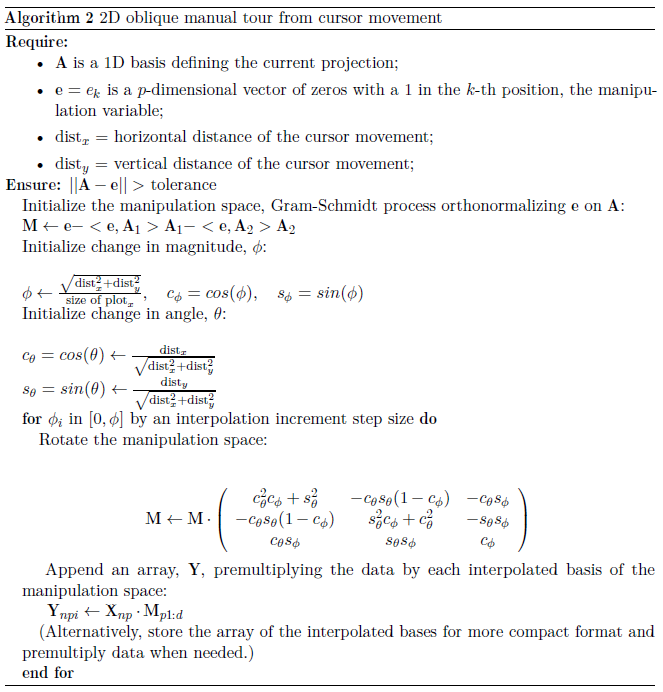
The chapter is organized as follows. Section 3.1 provides an illustrated detailed description of a 2D manual tour and fills in the previously absent details to solve the 3D rotation matrix used in 2D manual tours. This proves a scaffolding for the extension to solving a 4D rotation matrix for a 3D manual tour. Section 3.2 includes compact algorithms for capturing oblique movements from a cursor. Section 3.3 discusses the functions and code usage to perform radial tours and compose a layered display of tours. Section 3.4 illustrates a use case of the radial tour facilitating sensitivity analysis on high-energy physics experiments (Wang et al. 2018). Section 3.5 concluded with a discussion of this chapter.

3.1 Algorithm

The types of manipulations of the manual tour can be thought of in several ways:

• radial: fix the direction of contribution, and allow the magnitude to change.
• angular: fix the magnitude, and allow the angle direction of contribution to vary.
• horizontal, vertical: changing the contribution in horizontal or vertical directions.
• oblique: paths deviating from these movements, such as being captured by the movement of a cursor.

Angular manipulations are homomorphic in that they show the same information while rotating the frame. More interesting is a change in the magnitude of the contribution, changing the radius along the original contribution angle. For this reason, we implement the radial tour as the default for the manual tour. Below we describe the manual tour illustrated in detail. After that, the algorithms for oblique cursor movements in 1- and 2D are covered.

3.1.1 Notation

The notation used to describe the algorithm for a 2D radial manual tour is as follows:

• \(\textbf{X}\), the data, an \(n \times p\) quantitative matrix to be projected.
• \(\textbf{A}\), any orthonormal projection basis, \(p \times d\) matrix, describing the projection from \(\mathbb{R}^p \Rightarrow \mathbb{R}^d\).
• \(k\), is the index of the manipulation variable or manip var for short.
• \(\textbf{e}\), a 1D basis vector of length \(p\), with 1 in the \(k\)-th position and 0 elsewhere.
• \(\textbf{R}\), the \(d+1\)-D rotation matrix, performs unconstrained 3D rotations within the manip space, \(\textbf{M}\).
• \(\theta\), the angle of in-projection rotation, for example, on the reference axes; \(c_\theta, s_\theta\) are its cosine and sine.
• \(\phi\), the angle of out-of-projection rotation into the manip space; \(c_\phi, s_\phi\) are its cosine and sine. The initial value for animation purposes is \(\phi_1\).
• \(\textbf{U}\), the axis of rotation for out-of-projection rotation orthogonal to \(\textbf{e}\).
• \(\textbf{Y} = \textbf{X} \times \textbf{A}\), the resulting data projection through the manip space, \(\textbf{M}\), and rotation matrix, \(\textbf{R}\).

The algorithm operates entirely on projection bases and incorporates the data only when making the projected data plots in light of efficiency.

3.1.2 Steps

3.1.2.1 Step 0) Setup

The flea data (Lubischew 1962), available in the tourr package (Wickham et al. 2011), is used to illustrate the algorithm. The data contains 74 observations of six variables, each a physical measurement of the flea beetles. Each observation belongs to one of three species. Each variable is normalized to a common range of [0, 1].

An initial 2D projection basis must be provided. A suggested way to start is to identify an interesting projection using a projection pursuit guided tour. The holes index is used to find a 2D projection of the flea data, which shows three separated species groups. Figure 3.1 shows the initial projection of the data. On the left, a biplot (Gabriel 1971) illustrates the projection basis (\(\textbf{A}\)), showing each variable’s magnitude and direction of contribution to the projection. The right side shows the projected data, \(\textbf{Y}_{[n,~2]} ~=~ \textbf{X}_{[n,~p]} \textbf{A}_{[p,~2]}\). The color and shape of points are mapped to the flea species.

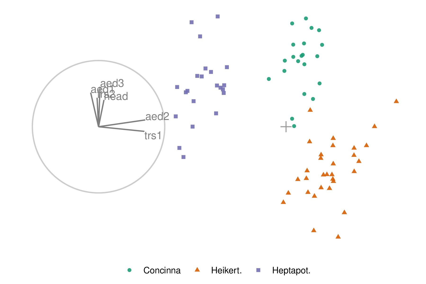
Figure 3.1: Biplot of the initial 2D projection of normalized flea data. The basis is depicted on the left, and the resulting data projection is on the right. The color and shape of data points are mapped to the flea beetle species. The basis was produced by a projection pursuit guided tour with the holes index. The contribution of the variables aede2 and tars1 approximately contrasts the other variables. The visible structure in the projection is the three species clusters.

3.1.2.2 Step 1) Choose manip variable

In figure 3.1, the variable contributions of tars1 and aede2 mostly contrast the other four variables. These two variables combined contribute in the direction where the purple cluster is separated from the other two clusters. The variable aede2 is selected as the manip var, whose contribution is changed. The aspect being explored is: how important is this variable to separating the clusters in this projection?

3.1.2.3 Step 2) Create the 3D manip space

Initialize a zero vector, \(\textbf{e}\), of length \(p\), and set the \(k\)-th element to 1. In the example data, aede2 is the fifth variable in the data, so \(k=5\), set \(e_5=1\). Append this vector to the current basis as the third column. Use a Gram-Schmidt process to orthonormalize the coordinate basis vector on the original 2D projection to describe a 3D manip space, \(\textbf{M}\).

\[\begin{align*} e_k &\leftarrow 1 \\ \textbf{e}^*_{[p,~1]} &= \textbf{e} - \langle \textbf{e}, \textbf{A}_1 \rangle \textbf{A}_1 - \langle \textbf{e}, \textbf{A}_2 \rangle \textbf{A}_2 \\ \textbf{M}_{[p,~3]} &= (\textbf{A}_1,\textbf{A}_2,\textbf{e}^*) \end{align*}\]

The manip space provides a 3D projection from \(p\)-dimensional space, where the coefficient of the manip var can range completely between [0, 1]. This 3D space serves as the medium to rotate the projection basis relative to the selected manipulation variable. Figure 3.2 illustrates this 3D manip space with the manip var highlighted. This representation is produced by calling the view_manip_space() function. This diagram is purely used to help explain the algorithm.

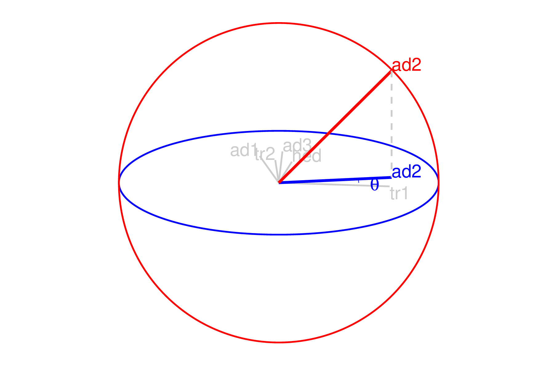
Figure 3.2: Illustration of a 3D manip space. The projection plane is shown as a blue circle extending into and out of the display. A manipulation direction is initialized, the red circle, orthogonal to the projection plane. This allows the selected variable, aede2, to change its contribution to the projection plane. The other variables’ contributions rotate into this space, preserving the orthogonal basis, but are omitted in the manipulation dimension for simplicity.

3.1.2.4 Step 3) Defining a 3D rotation

The basis vector corresponding to the manip var (red line in Figure 3.2) can be operated like a lever anchored at the origin. This manual control process rotates the manip variable into and out of the 2D projection (Figure 3.3). As the variable contribution is controlled, the manip space turns, and the projection onto the horizontal plane correspondingly changes. This is a manual tour. Generating a sequence of values for the rotation angles produces a path for the rotation of the manip space.

For a radial tour, fix \(\theta\), the angle describing rotation within the horizontal projection plane, and compute a sequence for \(\phi\), defining movement out of this plane. This will change \(\phi\) from the initial value, \(\phi_1\), the angle between \(\textbf{e}\) and its shadow in \(\textbf{A}\), to a maximum of \(0\) (manip var entirely in projection), then to a minimum of \(\pi/2\) (manip var orthogonal to the projection), before returning to \(\phi_1\).

Rotations in 3D can be defined by the axes they pivot on. Rotation within the projection, \(\theta\), is rotation around the \(Z\)-axis. Out-of-projection rotation, \(\phi\), is the rotation around an axis on the \(XY\) plane, \(\textbf{U}\), orthogonal to \(\textbf{e}\). Given these axes, the rotation matrix, \(\textbf{R}\), can be written as follows, using Rodrigues’ rotation formula (originally published in Rodrigues 1840):

\[\begin{align*} \textbf{R}_{[3,~3]} &= \textbf{I}_3 + s_\phi\*\textbf{U} + (1-c_\phi)\*\textbf{U}^2 \\ &= \begin{bmatrix} 1 & 0 & 0 \\ 0 & 1 & 0 \\ 0 & 0 & 1 \\ \end{bmatrix} + \begin{bmatrix} 0 & 0 & c_\theta s_\phi \\ 0 & 0 & s_\theta s_\phi \\ -c_\theta s_\phi & -s_\theta s_\phi & 0 \\ \end{bmatrix} + \begin{bmatrix} -c_\theta (1-c_\phi) & s^2_\theta (1-c_\phi) & 0 \\ -c_\theta s_\theta (1-c_\phi) & -s^2_\theta (1-c_\phi) & 0 \\ 0 & 0 & c_\phi-1 \\ \end{bmatrix} \\ &= \begin{bmatrix} c_\theta^2 c_\phi + s_\theta^2 & -c_\theta s_\theta (1 - c_\phi) & -c_\theta s_\phi \\ -c_\theta s_\theta (1 - c_\phi) & s_\theta^2 c_\phi + c_\theta^2 & -s_\theta s_\phi \\ c_\theta s_\phi & s_\theta s_\phi & c_\phi \end{bmatrix} \\ \end{align*}\]

where

\[\begin{align*} \textbf{U} &= (u_x, u_y, u_z) = (s_\theta, -c_\theta, 0) \\ &= \begin{bmatrix} 0 & -u_z & u_y \\ u_z & 0 & -u_x \\ -u_y & u_x & 0 \\ \end{bmatrix} = \begin{bmatrix} 0 & 0 & -c_\theta \\ 0 & 0 & -s_\theta \\ c_\theta & s_\theta & 0 \\ \end{bmatrix} \\ \end{align*}\]

3.1.2.5 Step 4) Creating an animation of the radial rotation

The steps outlined above can be used to create any arbitrary rotation in the manip space. In the radial tour, the manip var is rotated fully into the projection, completely out, and then back to the initial value. This involves varying \(\phi\) between \(0\) and \(\pi/2\), call the steps \(\phi_i\).

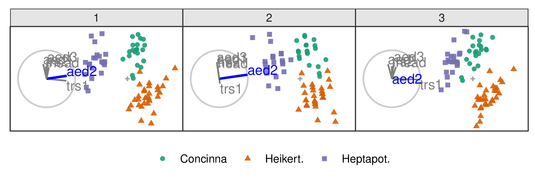
Figure 3.3: Select frames of a radial tour manipulating aede2: (1) original projection, (2) full contribution, (3) zero contribution. After zeroing the contribution the animation continues to return to the initial contribution.

1. Set the initial value of \(\phi_1\) and \(\theta\): \(\phi_1 = \cos^{-1}{\sqrt{A_{k1}^2+A_{k2}^2}}\), \(\theta = \tan^{-1}\frac{A_{k2}}{A_{k1}}\). Where \(\phi_1\) is the angle between \(\textbf{e}\) and its shadow in \(\textbf{A}\).
2. Set an angle increment (\(\Delta_\phi\)), the step size between interpolated frames. The package spinifex uses an angle increment rather than the number of frames to control the movement to be consistent with the tour algorithm implemented in tourr.
3. Step towards \(0\), where the manip var is entirely in the projection plane.
4. Step towards \(\pi/2\), where the manip variable has no contribution to the projection.
5. Step back to \(\phi_1\).

In steps 3-5, a small step may be added to ensure that the endpoints of \(\phi\) (\(0\), \(\pi/2\), \(\phi_1\)) are reached.

3.1.2.6 Step 5) Projecting the data

The operation of a manual tour is defined on the projection bases. The data is projected through the relevant bases only when the presentation is needed.

\[\begin{align*} \textbf{Y}^{(i)}_{[n,~3]} &= \textbf{X}_{[n,~p]} \textbf{M}_{[p,~3]} \textbf{R}^{(i)}_{[3,3]} \end{align*}\]

where \(\textbf{R}^{(i)}_{[3,3]}\) is the incremental rotation matrix, using \(\phi_i\). To make the data plot, use the first two columns of . Show the projected data for each frame in sequence to form an animation.

Tours are typically viewed as animation. The animation of this tour can be viewed online on GitHub.

3.2 Oblique cursor movement

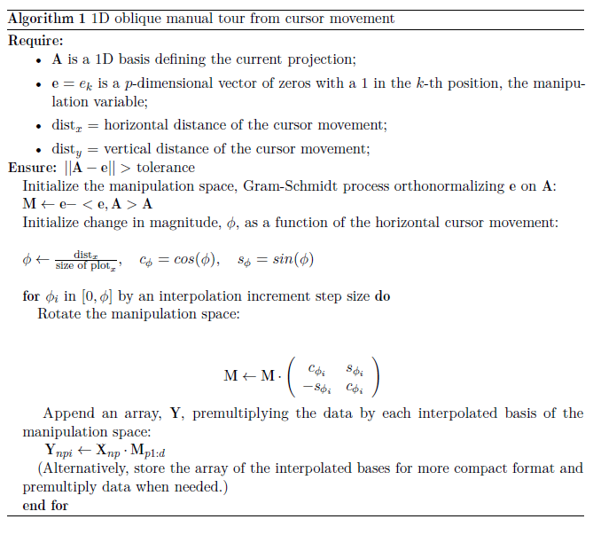
In a move abbreviated way, we can think about the algorithm for 1D and 2D oblique manual tours as:

3.3 Package structure

In addition to facilitating the manual tour, the other primary function of the spinifex package facilitates the layered composition of tours interoperably with tours from tourr. This package attempts to abstract the complexity of dealing with an unknown number of frames and replicating the length of arguments. We use a layered composition approach to tours similar to ggplot2 (Wickham 2016). The resulting displays are then animated with plotly (Sievert 2020) or gganimate (Pedersen and Robinson 2020). This section describes the functions available in the package, their usage, and how to install and get up and running.

3.3.1 Usage

The penguins data (Gorman et al. 2014; Horst et al. 2020), also available in spinifex, is used to illustrate the creation of a radial tour, layered composition, and animation. Like the flea data, this explores the variable contribution that leads to the separation of clusters.

library(spinifex)

## Process penguins data
dat  <- scale_sd(penguins_na.rm[1:4])
clas <- penguins_na.rm$species

## Start basis and  manual tour path
bas     <- basis_olda(data = dat, class = clas)
mt_path <- manual_tour(basis = bas, manip_var = 1, data = dat)

## Compose the tour display
ggt <- ggtour(mt_path, angle = .15) +
  proto_point(aes_args      = list(color = clas, shape = clas),
              identity_args = list(alpa = .8, size = 1.5)) +
  proto_basis() +
  proto_origin()

## Animate
animate_plotly(ggt, fps = 5)

Composition and animation options are interoperable with tourr produced tours. The code below similarly composes a 1D tour from a saved grand tour path.

## A grand tour from tourr
library(tourr)
gt_path <- save_history(data = dat, tour_path = grand_tour(), max_bases = 10)

## Compose 1D tour display
ggt2 <- ggtour(gt_path, angle = .15) +
  proto_density(aes_args = list(color = clas, fill = clas)) +
  proto_basis1d() +
  proto_origin1d()

## Animate
animate_plotly(ggt2, fps = 5)

3.3.2 Functions

Table 3.1 lists the primary functions and their purpose. These are grouped into four classes: processing the data, production of tour path, the composition of the tour display, and its animation.

Table 3.1: Summary of primary functions.

Family	Function	Related to	Description
processing	scale_01/sd		scale each column to [0,1]/std dev away from the mean
processing	basis_pca/olda/…	Rdimtools::do.*	basis of orthogonal component spaces
processing	basis_half_circle		basis with uniform contribution across half of a circle
processing	basis_guided	tourr::guided_tour	silently returns the basis from a guided tour
tour path	manual_tour		basis and interpolation information for a manual tour
tour path	save_history	tourr::save_history	silent, extended wrapper returning other tour arrays
display	ggtour	ggplot2::ggplot	canvas and initialization for a tour animation
display	proto_point/text	geom_point/text	adds observation points/text
display	proto_density/2d	geom_density/2d	adds density curve/2d contours
display	proto_hex	geom_hex	adds hexagonal heatmap of observations
display	proto_basis/1d		adds adding basis visual in a unit-circle/-rectangle
display	proto_origin/1d		adds a reference mark in the center of the data
display	proto_default/1d		wrapper for proto_* point + basis + origin
display	facet_wrap_tour	ggplot2::facet_wrap	facets on the levels of variable
display	append_fixed_y		add/overwrite a fixed vertical position
animation	animate_plotly	plotly::ggplotly	render as an interactive hmtl widget
animation	animate_gganimate	gganimate::animate	render as a gif, mp4, or other video formats
animation	filmstrip		static ggplot faceting on the frames of the animation

3.3.3 Installation

The spinifex is available from CRAN. The following code will help to get up and running:

# Installation:
install.package("spinifex") ## Install from CRAN
library("spinifex") ## Load into session

# Getting started:
## Shiny app for visualizing basic application
run_app("intro")
## View the code vignette
vignette("getting_started_with_spinifex")
## More about proto_* functions
vignette("ggproto_api")

3.4 Use cases

Wang et al. (2018) introduce a new tool, PDFSense, to visualize the sensitivity of hadronic experiments to nucleon structure. The parameter space of these experiments lies in 56 dimensions which is approximated as the ten first principal components.

Cook et al. (2018) illustrate using the grand tour to explore this component-reduced space. Tours can better resolve the shape of clusters, intra-cluster detail, and lead to better outlier detection than PDFSense, TFEP (TensorFlow embedded projections), or traditional static embeddings. We start from a basis identified with a grand tour in the previous work. From this basis we apply the manual tour to examine the sensitivity of a variable’s contribution to the structure in the projection.

The data has a hierarchical structure with top-level clusters; DIS, VBP, and jet. Each cluster is a particular class of experiments, and each observation is an aggregation of experiments. In consideration of data occlusion, we conduct manual tours on subsets of the DIS and jet clusters. This explores the structure’s sensitivity to each of the variables in turn. The subjectively most and least sensitive variables are illustrated for identifying the clusters’ dimensionality and describing the clusters’ range.

3.4.1 Jet cluster

The jet cluster resides in a smaller dimensionality than the full set of experiments, with four principal components explaining 95% of the variation in the cluster (Cook et al. 2018). The data within this 4D embedding is classified into ATLAS7old and ATLAS7new, focusing on two groups occupying different subspace locations. Radial tours controlling contributions from PC4 and PC3 are shown in Figures 3.4 and 3.5, respectively. The difference in shape can be interpreted as the experiments probing different phase spaces. Back-transforming the principal components to the original variables can be done for a more detailed interpretation.

When PC4 is removed from the projection (Figure 3.4), the difference between the two groups is removed, indicating that PC4 is essential for separating types of experiments. However, eliminating PC3 from the projection (Figure 3.5) does not affect the structure, meaning PC3 is not essential for distinguishing experiments. Animations varying the contributions of all components can be viewed at the following links: PC1, PC2, PC3, and PC4. It can be seen that only PC4 is vital for viewing the difference in these two experiments.

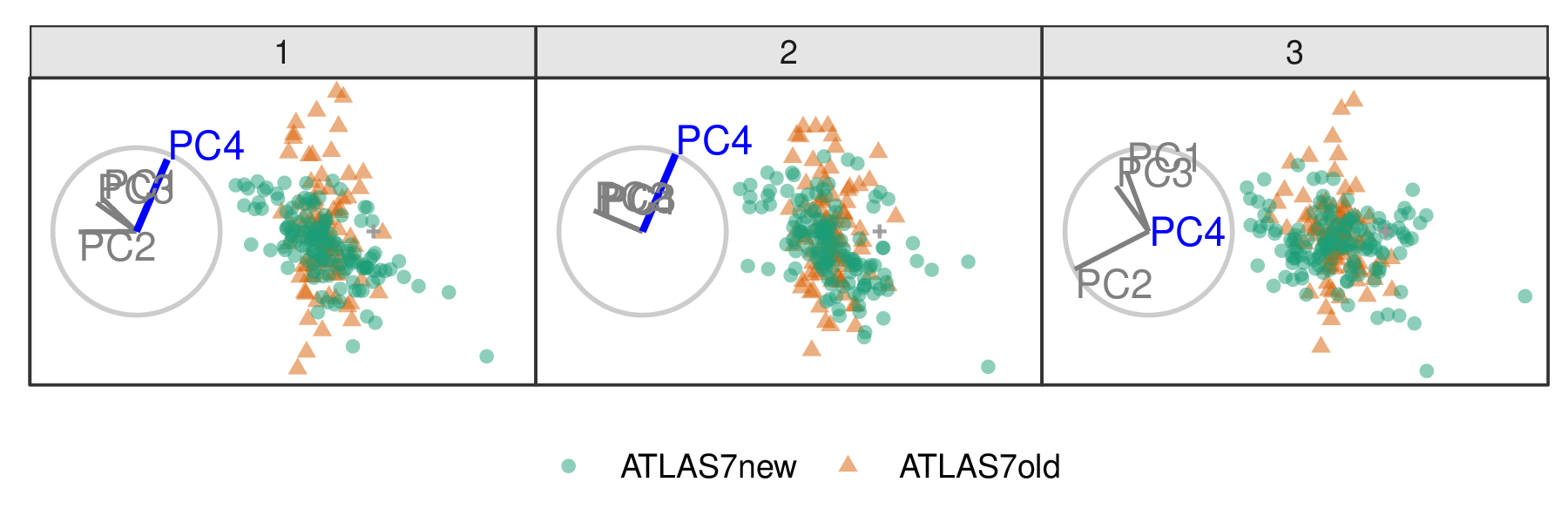
Figure 3.4: Select frames from a radial tour of PC4 within the jet cluster, with color indicating experiment type: ATLAS7new (green) and ATLAS7old (orange). When PC4 is removed from the projection (frame 10), and there is little difference between the clusters, suggesting that PC4 is vital for distinguishing the experiments.

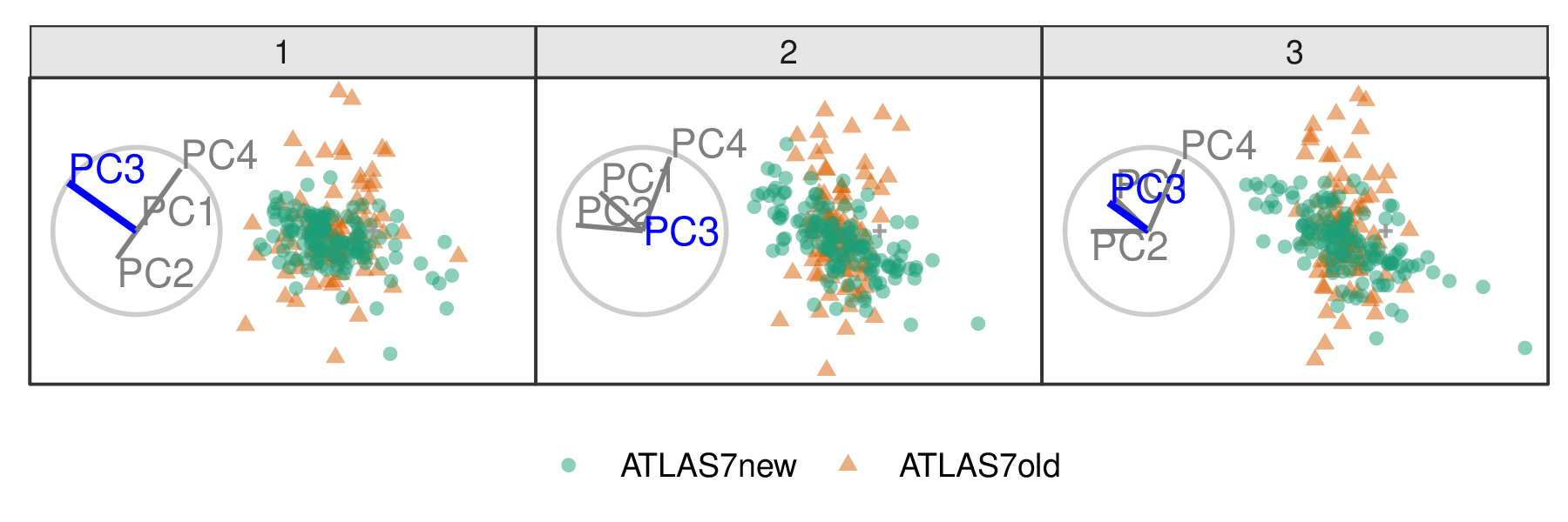
Figure 3.5: Frames from the radial tour manipulating PC3 within the jet cluster, with color indicating experiment type: ATLAS7new (green) and ATLAS7old (orange). When the contribution from PC3 is changed, there is little change in the separation of the clusters, suggesting that PC3 is not important for distinguishing the experiments.

3.4.2 DIS cluster

Following Cook et al. (2018), PCA is used to explore the DIS cluster. The first six principal components are used, containing 48% of the full sample variation. The contributions of PC6 and PC2 are explored in Figures 3.6 and 3.7, respectively. Three experiments are examined: DIS HERA1+2 (green), dimuon SIDIS (purple), and charm SIDIS (orange).

Both PC2 and PC6 contribute to the projection similarly. When PC6 is rotated into the projection, variation in the DIS HERA1+2 is greatly reduced. When PC2 is removed from the projection, dimuon SIDIS becomes more distinct. Even though both variables contribute similarly to the original projection, their contributions have quite different effects on the structure of each cluster and the distinction between clusters. Animations of all of the principal components can be viewed from the links: PC1, PC2, PC3, PC4, PC5, and PC6.

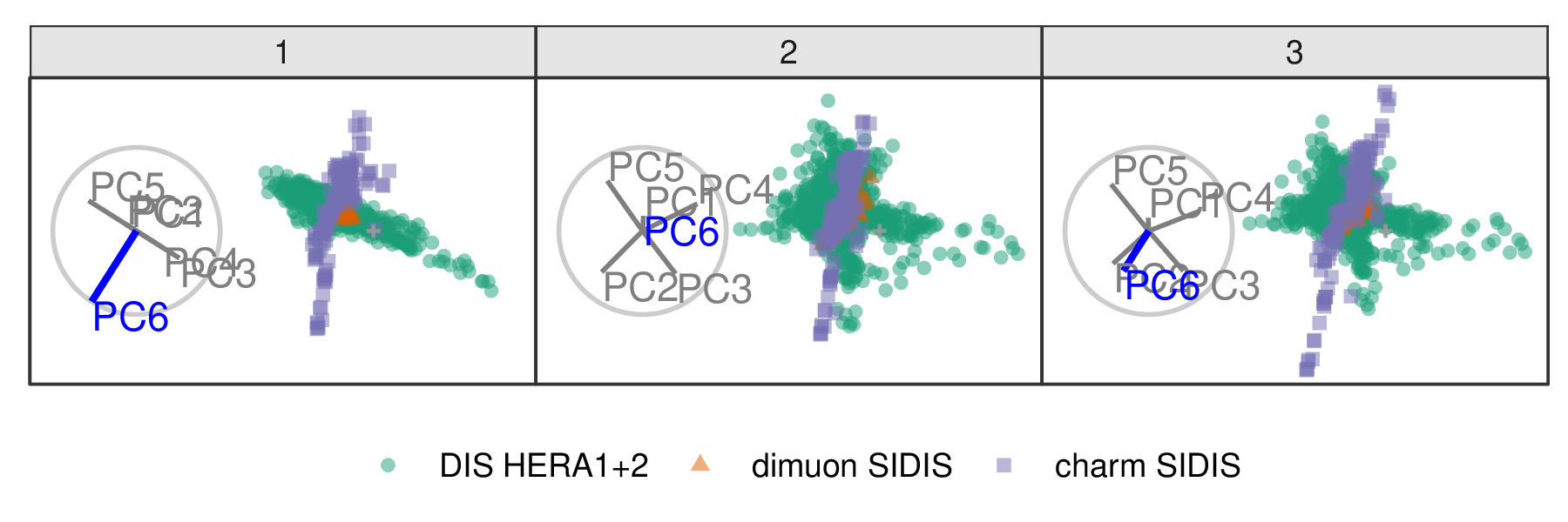
Figure 3.6: Select frames from a radial tour exploring the sensitivity that PC6 has on the structure of the DIS cluster, with color indicating experiment type: DIS HERA1+2 (green), dimuon SIDIS (purple), and charm SIDIS (orange). DIS HERA1+2 is distributed in a cross-shape, with charm SIDIS occupying the center. Dimuon SIDIS is a linear cluster crossing DIS HERA1+2. As the contribution of PC6 is increased, DIS HERA1+2 becomes almost singular in one direction (frame 5), indicating that this cluster has minimal variability in the direction of PC6.

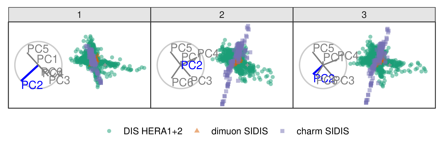
Figure 3.7: Frames from the radial tour exploring the sensitivity PC2 to the structure of the DIS cluster, with color indicating experiment type: DIS HERA1+2 (green), dimuon SIDIS (purple), and charm SIDIS (orange). As the contribution of PC2 is decreased, dimuon SIDIS becomes more distinguishable from the other two clusters, indicating that the absence of PC2 is vital for separating this cluster from the others.

3.5 Discussion

Dynamic linear projections of quantitative multivariate data, tours, play an essential role in data visualization; they extend the dimensionality of visuals to peek into high-dimensional data and parameter spaces. This research has taken the manual tour algorithm, specifically the radial rotation, used in GGobi (Swayne et al. 2003) to interactively rotate a variable into or out of a 2D projection and modified it to create an animation that performs the same task. It is most helpful in examining the importance of variables and how the structure in the projection is sensitive or not to specific variables. This functionality is made available in the package spinifex. Which also extends the geometric display and export formats interoperable with the tourr package.

The original conception of the grand tour was motivated by problems in physics (Asimov 1985). Thus, the use case was fitting. The radial tour was used to explore the sensitivity of variable contributions to the separation of different experiments in high-energy particle physics. These tools can be applied quite broadly to many multivariate data analysis problems.

The manual tour is constrained because the effect of one variable depends on the contributions of other variables in the manip space. However, this can simplify a projection by removing variables without affecting the visible structure. Defining a manual rotation in high dimensions is possible using Givens rotations and Householder reflections as outlined by Buja et al. (2005). This would provide more flexible manual rotation but more difficult for a user because they have the choice (too much choice) of which directions to move.