B Supplementary material
Below collects links to documentation, code vignettes, and animations related to the content. The content for Chapter 4, continues with a bit of an extended analysis looking at the visual displays in the user study, the participant demographics, and a parallel analysis regressing of log time.
B.1 Thesis
| Content | Link |
|---|---|
| thesis repository | https://tinyurl.com/bddbs6sr |
| thesis, pdf format | https://tinyurl.com/5c54s7bf |
| thesis, html format | https://tinyurl.com/2p8m92bs |
| Penguins radial tour, Figure 1.2 | https://vimeo.com/676723431 |
| Penguins grand tour, Figure 2.4 | https://vimeo.com/676723441 |
B.2 Chapter 3, spinifex links
| Content | Link |
|---|---|
| spinifex documentation website | https://tinyurl.com/2p82e782 |
| Vignette: Getting started with spinifex | https://tinyurl.com/2p98cfwh |
| Vignette: Ggproto api | https://tinyurl.com/2p8m6cmc |
| Fleas, radial tour animation, Figure 3.3 | https://tinyurl.com/3t6w7psf |
| Jet cluster, varying PC1 | https://tinyurl.com/ye252yxb |
| Jet cluster, varying PC2 | https://tinyurl.com/ye252yxb |
| Jet cluster, varying PC3, Figure 3.5 – least sensitive | https://tinyurl.com/4wv3j92k |
| Jet cluster, varying PC4, Figure 3.4 – most sensitive | https://tinyurl.com/yckwdb5s |
| DIS cluster, varying PC1 | https://tinyurl.com/2wz377vh |
| DIS cluster, varying PC2, Figure 3.7 – least sensitive | https://tinyurl.com/2hrxfdje |
| DIS cluster, varying PC3 | https://tinyurl.com/ms683n2e |
| DIS cluster, varying PC4 | https://tinyurl.com/yhm244f7 |
| DIS cluster, varying PC5 | https://tinyurl.com/4p5n3s77 |
| DIS cluster, varying PC6, Figure 3.6 – most sensitive | https://tinyurl.com/mvcn2a8v |
B.3 Chapter 4, user study extended analysis
This section covers extended analysis. First, it illustrations of the different visuals are provided. Then, the participant demographics are covered. Lastly, a parallel modeling analysis on log response time is conducted.
B.3.1 Visual methods
Below illustrates the three visual methods evaluated in the user study. Data was collected from a shiny application and pre-rendered gif files were displayed based on the selected inputs. The instructional video that the participants were shown at the start of the study can be viewed at https://vimeo.com/712674984.
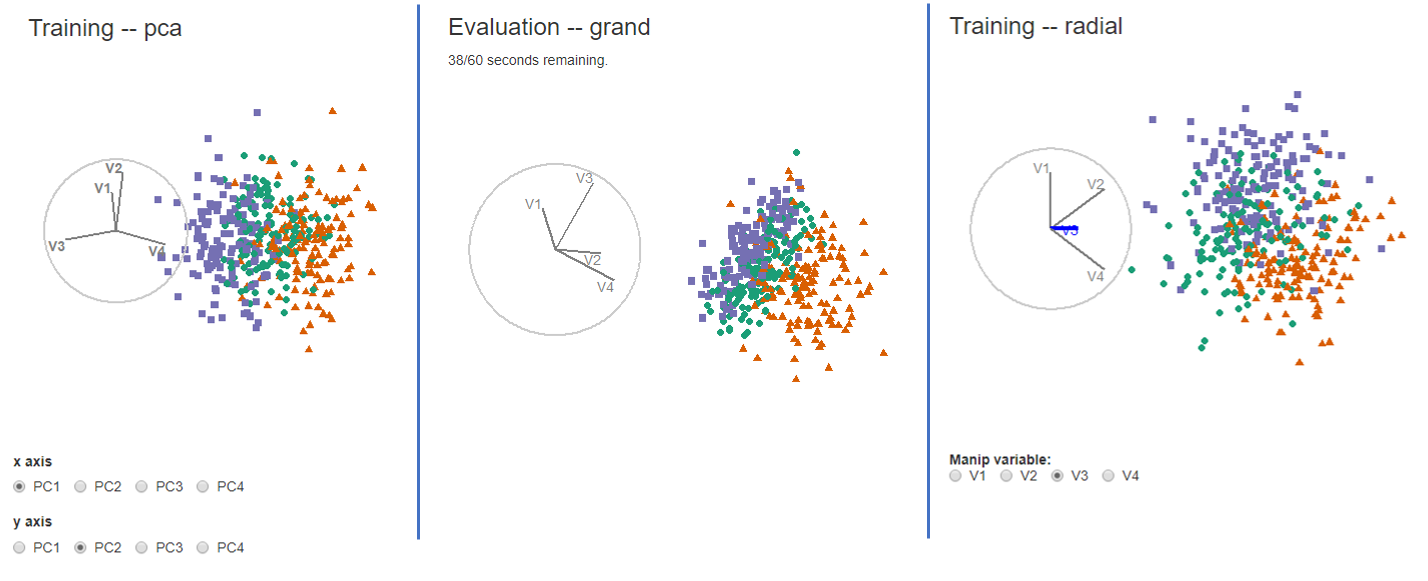
Figure B.1: Examples of the application displays for PCA, grand tour, and radial tour.
B.3.2 Survey participant demographics
The target population is relatively well-educated people, as linear projections may prove difficult for generalized consumption. Hence Prolific.co participants are restricted to those with an undergraduate degree (58,700 of the 150,400 users at the study time). From this cohort, 108 performed a complete study. Of these participants, 84 submitted the post-study survey, represented in the following heatmap. All participants were compensated for their time at 7.50 per hour, with a mean time of about 16 minutes. Figure B.2 shows a heat map of the demographics for these 84 participants.
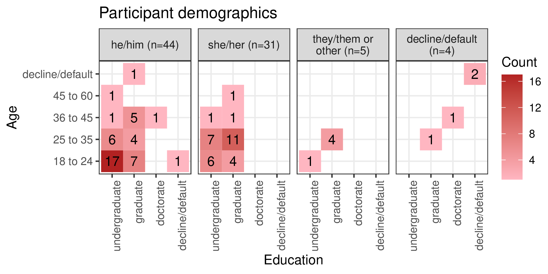
Figure B.2: Heatmaps of survey participant demographics; counts of age group by completed education as faceted across preferred pronouns. Our sample tended to be between 18 and 35 years of age with an undergraduate or graduate degree.
B.3.3 Response time
As a secondary explanatory variable, response time is considered. Response time is first log-transformed to remove its right skew. The same modeling procedure is repeated for this response. 1) Compare the performance of a battery of all additive and multiplicative models. Table B.1 shows the higher-level performance of these models over increasing model complexity. 2) Select the model with the same effect terms, \(\alpha \times \beta + \gamma + \delta\), with relatively high conditional \(R^2\) without becoming overly complex from interaction. The coefficients of this model are displayed in Table B.2.
| Fixed effects | No. levels | No. terms | AIC | BIC | R2 cond. | R2 marg. | RMSE |
|---|---|---|---|---|---|---|---|
| a | 1 | 3 | <span style=" font-weight: bold; " >1448</span> | <span style=" font-weight: bold; " >1475</span> | 0.645 | 0.007 | 0.553 |
| a+b+c+d | 4 | 8 | 1467 | 1516 | 0.647 | 0.017 | 0.552 |
| a*b+c+d | 5 | 12 | 1474 | 1541 | 0.656 | 0.024 | 0.548 |
| a*b*c+d | 8 | 28 | 1488 | 1627 | 0.673 | 0.054 | 0.536 |
| a*b*c*d | 15 | 54 | 1537 | 1792 | <span style=" font-weight: bold; " >0.7</span> | <span style=" font-weight: bold; " >0.062</span> | <span style=" font-weight: bold; " >0.523</span> |
| Estimate | Std. Error | df | t value | Pr(>|t|) | ||
|---|---|---|---|---|---|---|
| (Intercept) | 2.71 | 0.14 | 42.6 | 19.06 | 0.000 | *** |
| Visual | ||||||
| Visualgrand | -0.23 | 0.12 | 567.6 | -1.97 | 0.049 |
|
| Visualradial | 0.16 | 0.12 | 573.5 | 1.34 | 0.181 | |
| Fixed effects | ||||||
| Location33/66% | 0.05 | 0.14 | 40.9 | 0.34 | 0.737 | |
| Location50/50% | -0.05 | 0.14 | 42.1 | -0.35 | 0.729 | |
| ShapeEEV | -0.15 | 0.09 | 8.3 | -1.61 | 0.145 | |
| Shapebanana | -0.13 | 0.09 | 8.3 | -1.42 | 0.192 | |
| Dim6 | 0.14 | 0.08 | 8.3 | 1.90 | 0.093 | |
| Interactions | ||||||
| Visualgrand:Location33/66% | 0.24 | 0.18 | 580.9 | 1.34 | 0.181 | |
| Visualradial:Location33/66% | -0.24 | 0.18 | 582.4 | -1.32 | 0.188 | |
| Visualgrand:Location50/50% | 0.12 | 0.18 | 578.6 | 0.69 | 0.491 | |
| Visualradial:Location50/50% | 0.05 | 0.18 | 584.4 | 0.25 | 0.800 | |
B.4 Chapter 5, cheem links
| Content | Link |
|---|---|
| cheem documentation website | https://tinyurl.com/4avspber |
| Vignette: Getting started with cheem | https://tinyurl.com/2p85sm4c |
| cheem view application | https://tinyurl.com/2hubrts7 |
| Penguins animation, Figure 5.4 | https://vimeo.com/666431172 |
| Chocolates, animation, Figure 5.6 | https://vimeo.com/666431143 |
| Chocolates2, animation, Figure 5.7 | https://vimeo.com/666431148 |
| FIFA 2020, animation, Figure 5.8 | https://vimeo.com/666431163 |
| Ames house prices, animation, Figure 5.9 | https://vimeo.com/666431134 |